Part 2: Implementing service features

Introduction

This is the second part of the three-part series on HyperCLOVA. In this post, I'll talk about how we implemented service features using HyperCLOVA. First, let me introduce Early Stop, a feature we implemented to deliver faster responses to users with NAVER's HyperCLOVA-based service patterns, such as CLOVA AI Speaker. Second, I'll explain how we were able to provide Semantic Search, a feature that analyzes the relevance between documents using a sentence generation model called the HyperCLOVA Model. And finally, I'll talk about P-tuning, a feature we implemented to achieve higher performance with the same model size in the serving environment. Here's the table of contents:

• Early Stop
• Semantic Search
• P-tuning

Early Stop

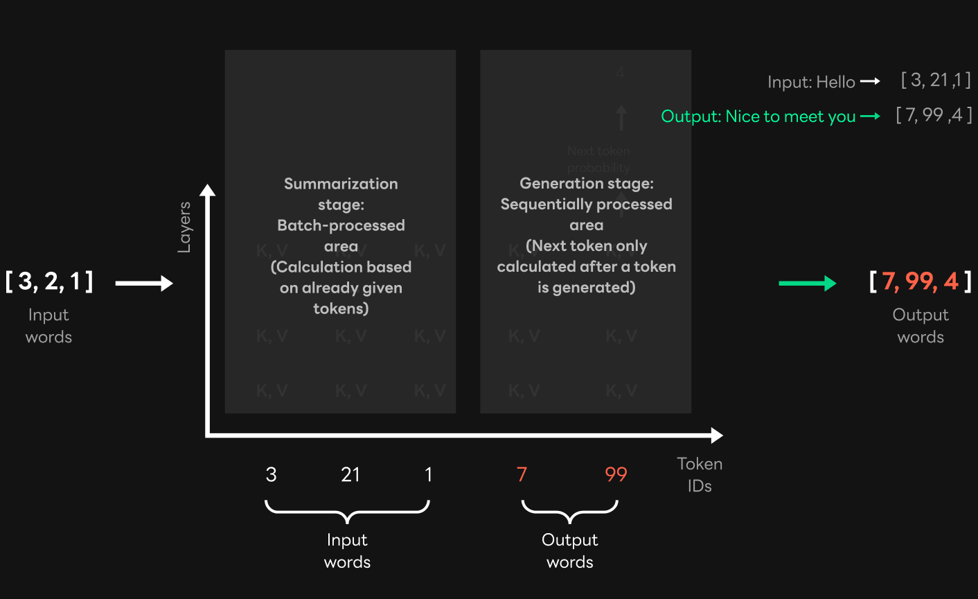
The most time-consuming step in a GPT-3 model such as HyperCLOVA is sentence generation. Due to the structural characteristics, transformer computation consists of two steps: a summarization step for processing input sentences and a generation step for generating sentences. In the summarization step, token IDs corresponding to input sentences are processed in batches simultaneously, while in the generation step, tokens are sequentially generated one by one. Therefore, the sentence generation step is responsible for the largest portion of the total computation time and reducing sentence length will directly reduce the response time. Then, how can you reduce sentence length in this step?

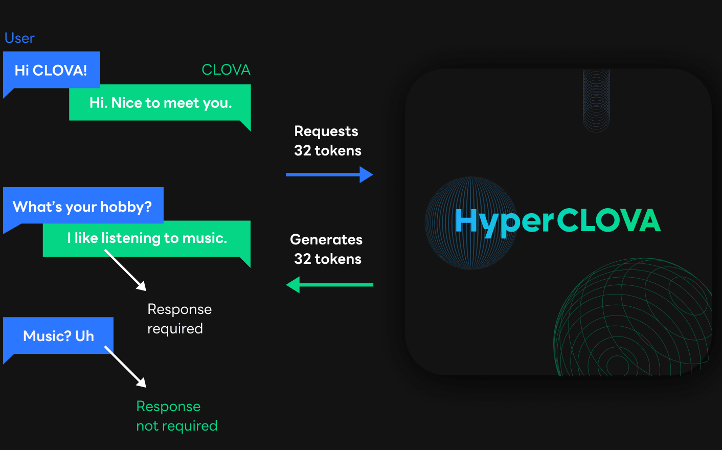
The figure above is an example where CLOVA AI Speaker requests HyperCLOVA to generate sentences. Based on the previous question of the conversation between CLOVA and the user in the upper-left corner, CLOVA AI Speaker asks HyperCLOVA to generate a sentence. At this time, the length of the sentence to be generated is also indicated as the number of tokens. HyperCLOVA generates tokens based on the requested length, converts them into sentences and then sends a response to CLOVA AI Speaker.

At this point, the requesting party has no idea how much HyperCLOVA will generate until it actually receives an answer. Therefore, a request allows a sufficient number of tokens for sentence generation, and only the part that user needs can be used as a response. In the example, the user only needs the sentence that starts with CLOVA: Thus, the sentence that starts with User: will be cut off, and only the first sentence will be used for the answer.

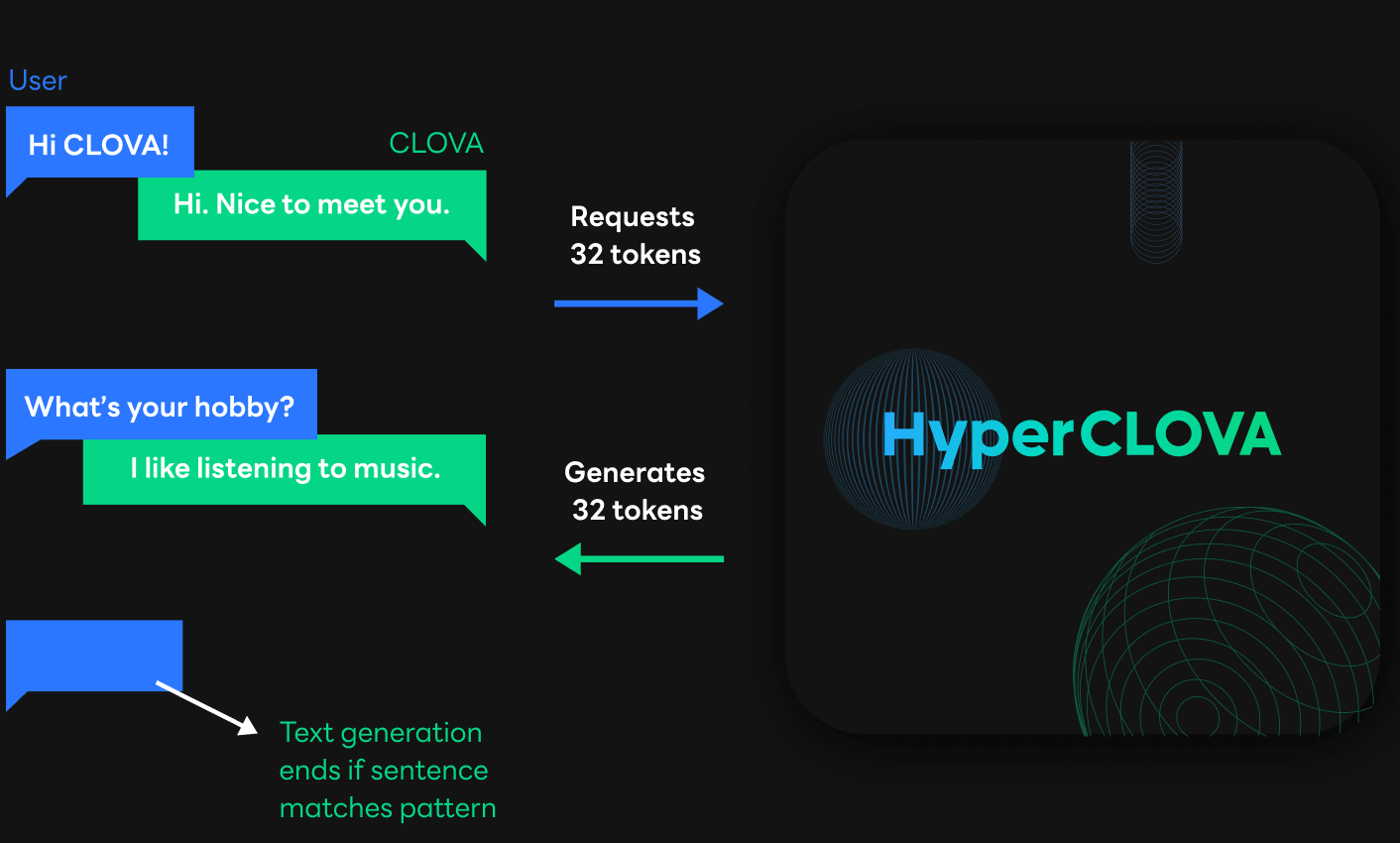
If HyperCLOVA generates and returns only the sentence that the user needs when generating sentences as shown in the figure below, it can reduce the sentence generation time, which accounts for the largest portion of the total latency, and also greatly reduce the response time. This feature is called Early Stop.

However, for HyperCLOVA with FasterTransformer as a transformer framework, we could not directly implement the Early Stop feature. In order to implement Early Stop, we needed a process to convert the generated token ID into a string every time to check if it matched the string for termination. This is because FasterTransformer, which is provided in the form of a shared library after compilation, can only be used with a set interface. It can only receive the results after the token IDs are generated based on the requested length.

To address this issue, we added a tokenizer for Early Stop in FasterTransformer and an interface to handle it to allow the generated token ID to be changed to a string every time.

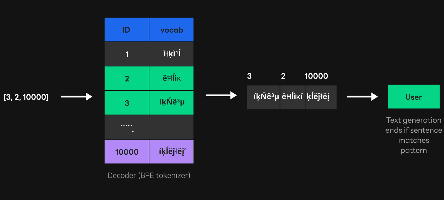
What we needed was a function to convert token IDs into strings, so we only implemented the decoder part of the tokenizer. In this case, the decoder part can be implemented using a simple hash map, because the information mapped with the Unicode corresponding to each token ID can be moved to the hash map as-is. The figure above shows the process of converting the token ID [3, 2, 10000] to the "User" string using the decoder of the tokenizer. By indexing the vocab mapped to each token ID and combining the Unicode found, the token ID can be converted to a string.

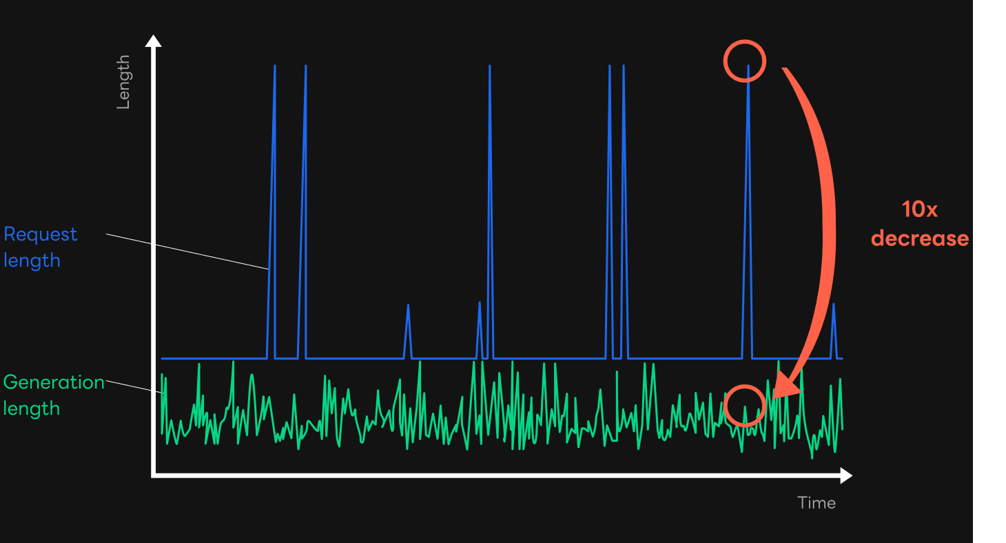
The figure above shows a graph where a log was kept and analyzed for the length of the requested sentence and the length of the sentence actually generated after the Early Stop feature was implemented. The blue line represents the requested length, and the green line represents the length of the generated sentence. Here you can see that the requested length was much longer than the length of the generated sentence in the service. In extreme cases, the latter was more than 10 times shorter than the former. In this case, it was also confirmed that the actual response time was reduced by nearly 10 times.

Semantic Search

GPT-3 models, such as HyperCLOVA, are essentially very suitable for processing sentence generation tasks. However, if you look closely at the principles of sentence generation, you can see that it can also be used for other purposes. In this section, we will summarize how HyperCLOVA can handle the task of semantic search and how we can set up the computational process.

What is Semantic Search? Semantic search is the process of inferring the context and relevance of input sentences or words and scoring them. Semantic search can be used to build a recommendation system using the relevance between sentences and words, and can also be used to evaluate if the trained model selects words of appropriate quality.

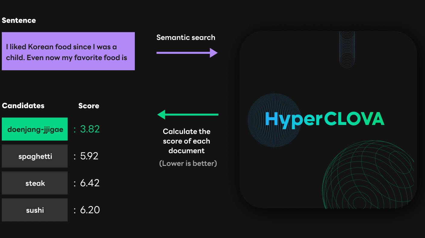
As shown in the example below, the semantic search feature calculates the relevance between the basic sentences and the candidate sentences as a score when they are added as input sentences. The higher the relevance between the basic sentences and the candidate sentences, the lower the score. In the example below, it was inferred that among the sentences in the candidate group, "doenjang-jjigae" has the highest relevance with the basic sentence.

Now let's compare the process of generating sentences in HyperCLOVA with the process of a semantic search.

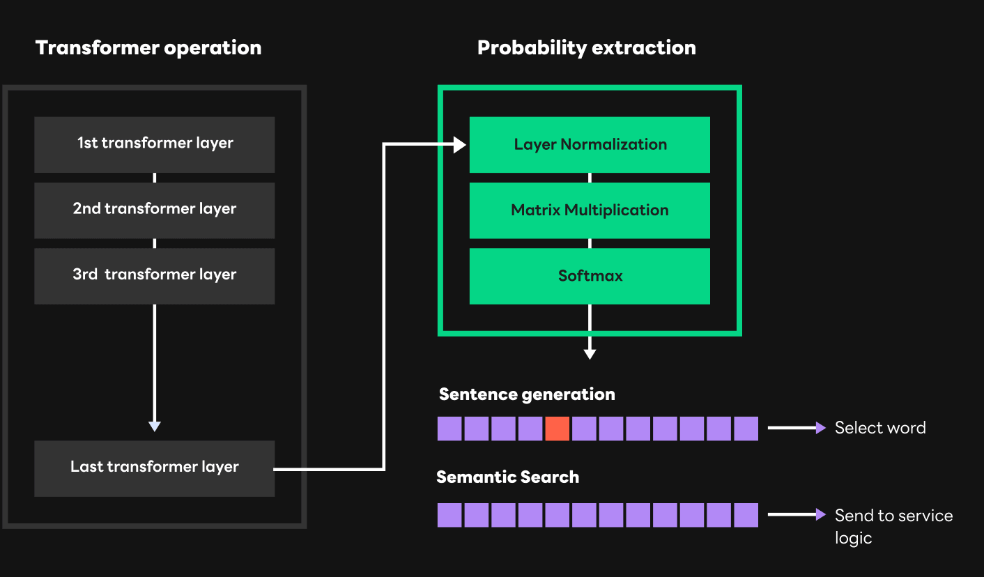
First, let's look at how these two processes are performed. GPT models, such as HyperCLOVA, basically compute using multiple transformer layers. These transformer layers use the concepts of query, key, and value. Query is related to the token currently given, and key and value are related to the entire sentence flow. In each transformer layer, computations using query, key, and value are sequentially performed one by one from the first layer to the last layer. Vectors are produced as a result of computations with query, key, and value, and using these values called "Hidden state" in the last layer, the probability of each word suitable for the next location can be extracted. The extraction process is as shown in the figure below. For the Hidden state in the last layer, LayerNorm (Layer Normalization), matrix multiplication with embedding table values, and Softmax are performed.

Once the probability of each word is extracted, the sentence generation and semantic search processes are performed slightly differently. The sentence generation step selects a word through a process called sampling using these probabilities. It can simply choose the word with the highest probability among many words, or randomly select from a few words with high probability by penalizing or giving random characteristics so that existing words are not generated. On the other hand, a semantic search must gather the probabilities of candidate words at each location among the extracted probabilities. Using these probabilities, it can infer which candidate word or sentence is most relevant to the basic sentence.

What was essential to provide a semantic search was adding this probability extraction part in the FasterTransformer framework. We modified the framework so that FasterTransformer can deliver the results of the probability calculation to service logic and implemented service logic so that it can proceed with the score calculation required by semantic search using these probabilities.

As we covered in the Early Stop section, when calculating probabilities, GPT computations are largely divided into a summarization stage, in which input sentences and words are processed in batches simultaneously, and a generation stage, in which the next words are generated one by one. The generation step is the process of extracting probabilities using keys and values in the previous word location and generating words one by one.

At first, we wrote the code so that probabilities were extracted through the computations in the generation step and then sent to service logic for a search score calculation. However, this method had a problem. In the generation step, serialized computations must be performed to extract the probability of each word, and this inevitably leads to greater latency.

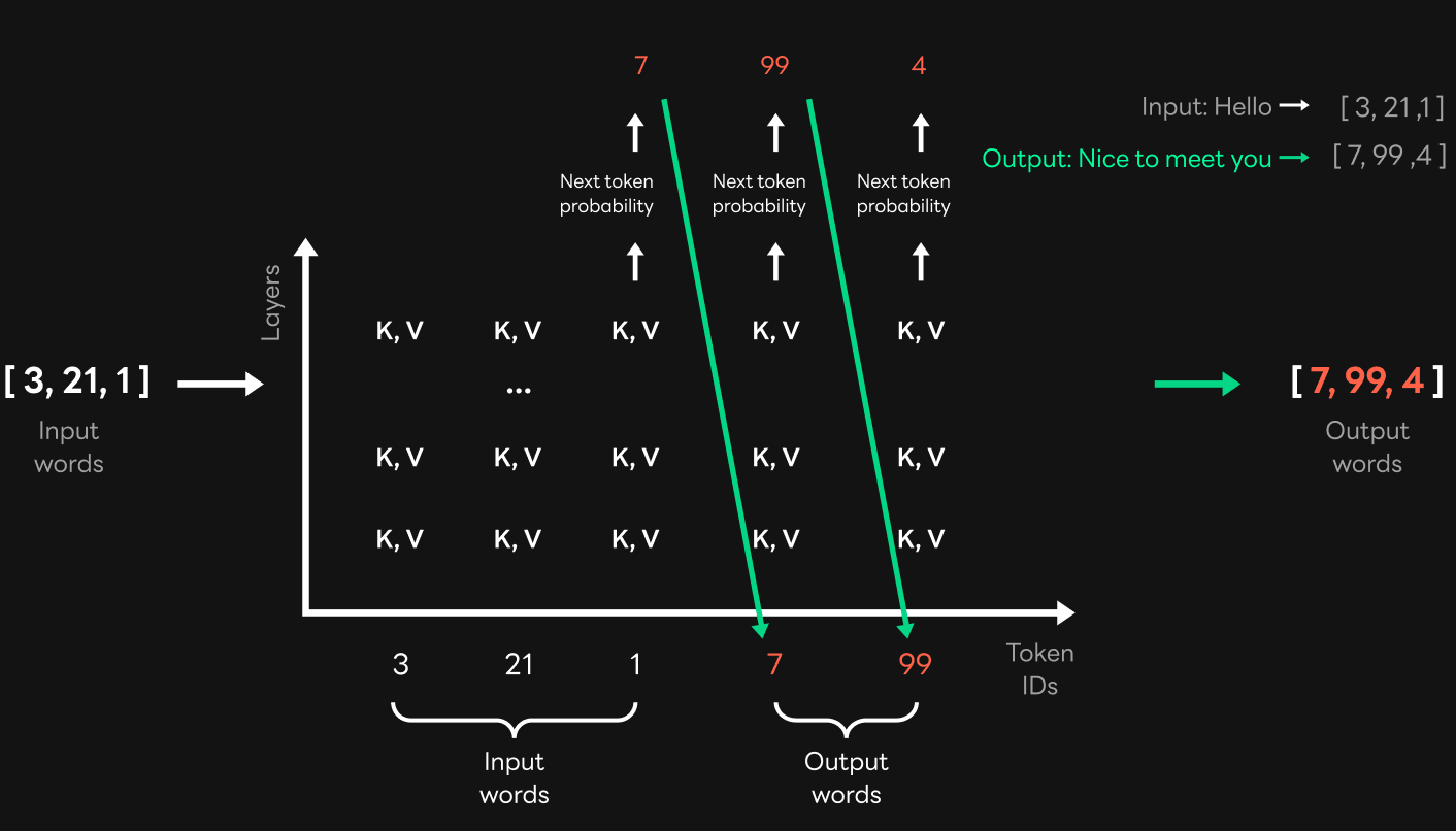
So we thought about how we could perform probability extractions faster using the characteristics of GPT. Earlier, I explained that probabilities of input words can be computed at once in the summarization step of GPT. When running a semantic search for basic and candidate sentences, both are input sentences and the probability at the location in the candidate sentence can be calculated simultaneously, as shown in the figure below.

So by extracting probabilities all at once in the summarization step, we were able to reduce the latency more than 10 times by using specific input sentences and candidate sentences for semantic searches. If we understood the GPT computations from the start, we could have designed the process like this in the first place. Unfortunately, we didn't think of this method at first, and we were able to come up with this optimization method only after we understood the structure of GPT more deeply.

P-tuning

As mentioned in Part 1, GPT-3 models, such as HyperCLOVA, are large in size and have a large amount of computations, so they have greater inference latency than other AI models. Since low latency is important for a better service experience, CLOVA is taking various steps to reduce the latency. There are ways to reduce latency. We can optimize computations to shorten the inference time or raise model performance to use a smaller model. We chose the latter and decided to support P-tuning. P-tuning is a process of training prompts tailored to specific tasks based on pre-trained models. Here, a prompt is a selected text inserted into the input example, and it induces sentence generation that is more suitable for the specific task.

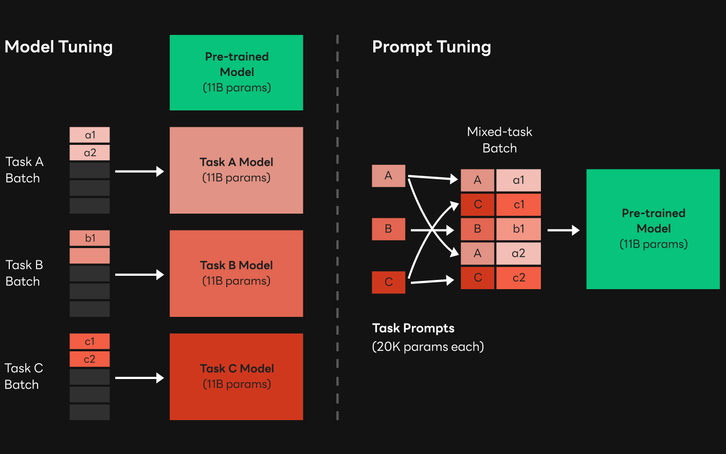
Compared to the fine tuning that we are familiar with, P-tuning is easier to understand. Suppose that we are planning various AI services for different tasks. In general, rather than training models suitable for each task from scratch, we use pre-trained models by tuning them to suit the situation. In this case, fine tuning is also called model tuning because model weight changes by training the pre-trained model for a relatively short time using a dataset suitable for each task. On the other hand, in P-tuning, the weight of the pre-trained model is not changed, and only the weight corresponding to the input prompt is trained. In general, prompt weight is much smaller than model weight, so P-tuning has a lower training burden and higher scalability than fine tuning. You can see these characteristics of P-tuning more clearly in large models such as GPT-3. The figure above shows the difference between model tuning and P-tuning.

To make the most of these advantages, the CLOVA Model Team planned to provide services with P-tuning and had to make preparations to support the feature in the serving environment. What things did we have to consider to support P-tuning in the serving environment instead of a model training environment? Since we had new inputs called "prompts," we needed to have them processed by the model. In order for the model to process these new inputs, we need to make sure the prompts are recognized by the model, and the weights corresponding to the recognized prompts are successfully sent to the model. First, let's take a closer look at the process of transferring input sentences to the transformer.

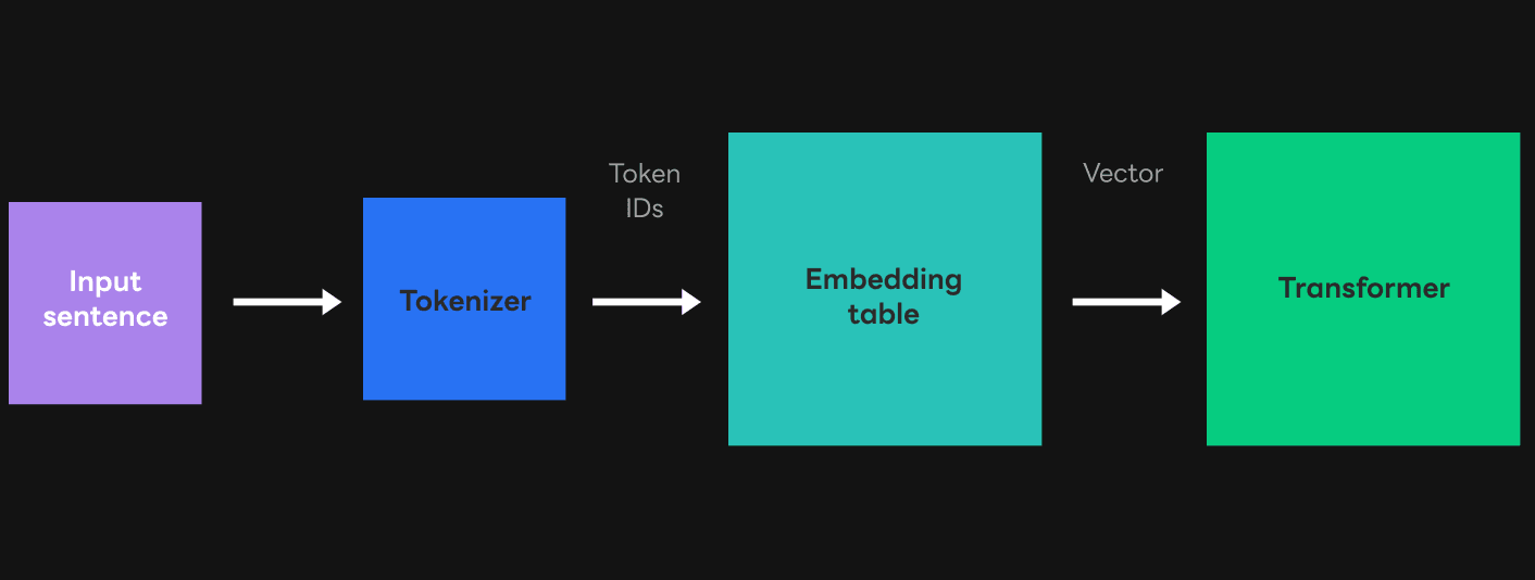
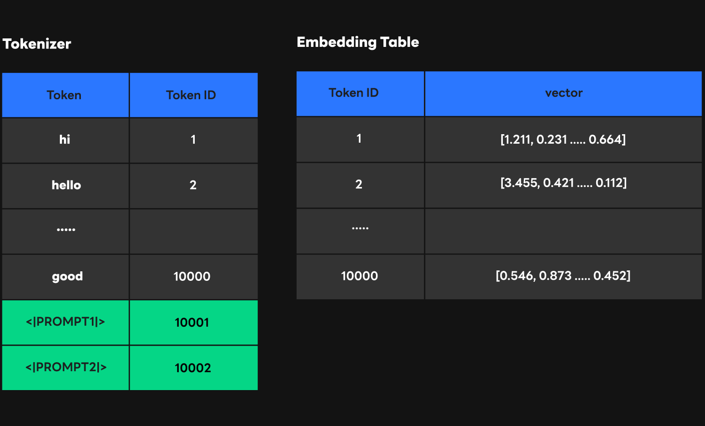
As shown in the figure above, the user sends strings when sending requests to HyperCLOVA, but since the transformer can only process vectors, we need a process to convert strings to vectors. As a result, input sentences are first changed to token IDs through the tokenizer, and token IDs are changed to vectors through the embedding table. In this process, token IDs act as a table offset. So by passing through the tokenizer and embedding table, inputs are converted to vectors that the transformer can recognize.

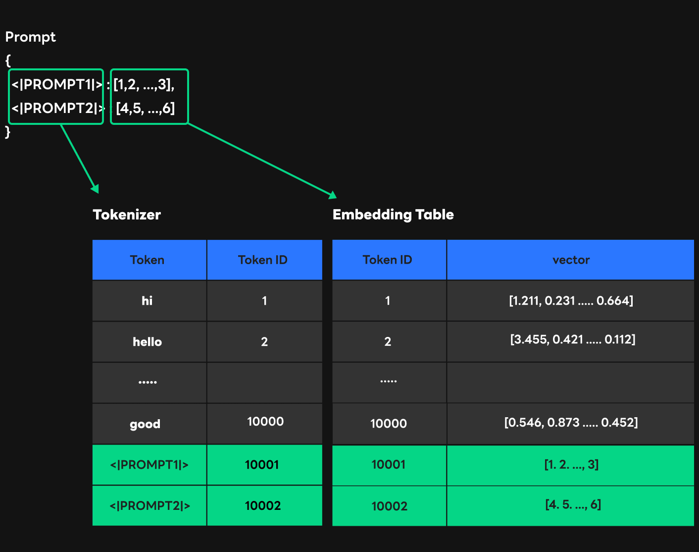
Then, how can we deliver prompt weight to the transformer for P-tuning? First, like with other string inputs, you should specify the string corresponding to the prompt and register it with the tokenizer so that it can be converted to a token ID. The Special Token function of the tokenizer allows you to register a string corresponding to the prompt at the end of the tokenizer. One thing of note is that the newly registered special token should be carefully selected so that it does not affect the existing tokens.

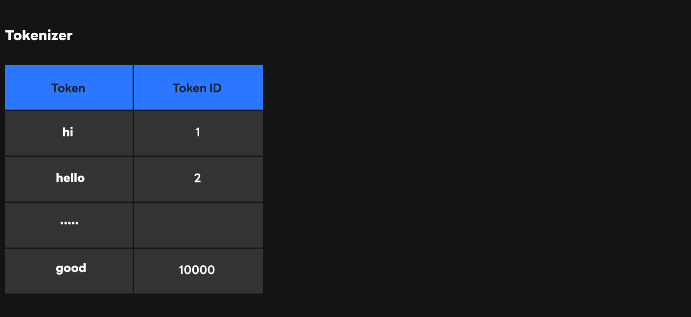
The figure above shows the tokenizer tokens and token IDs corresponding to the tokens. Let's assume that we are registering a prompt in the tokenizer. What happens if we set the token for this prompt as "hello"?

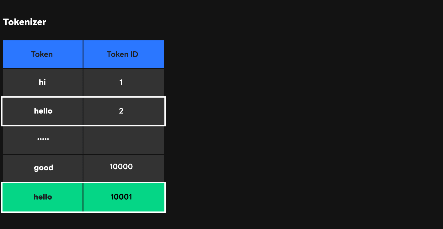
As shown in the figure, the token corresponding to "hello" is already registered as ID 2 in the tokenizer. However, if we register a new "hello" token for the prompt as a special token, "hello" will be given the last ID of tokenizer, 10001, and this makes it impossible to distinguish between the existing "hello" token and the prompt "hello" token. To prevent this issue, we set a special token(<|PROMPT|>) that would not overlap existing tokens and used it as a token for the prompt.

Then, how can we transfer the weight corresponding to the prompt to the transformer? We used two methods to do this. First, we registered the vector corresponding to the token ID in the embedding table. Second, we transferred the vector directly to the transformer at inference time.

1) First approach: Modifying the embedding table

The figure above shows how to modify the embedding table and deliver the prompt weight to the transformer. Earlier, I mentioned that the token ID that comes out as a result of tokenizer computation is used as the embedding table's offset. In other words, it means that if we add weight to the embedding table at this location when we have a token ID, it will work properly as expected. One thing to note here is that the prompt token ID added in this way should not be output as a result of transformer computation. However, due to the transformer's computational structure, there is a possibility that the token ID corresponding to the prompt will be output because computation with the embedding table is performed when the next token ID is selected. To prevent this, we set a variable called sampling size so that token can only be selected within that range.

There were two advantages to this method. First is the convenience in implementation. FasterTransformer is based on CUDA, so it takes a long time to modify and verify the code, but we can quickly implement the embedding table in Python because it only needs to modify the weight that exists as a file. Second is the cache effect. The weight belonging to the embedding table resides in the GPU memory, and the CUDA core has the fastest access to it. Since we registered the weight corresponding to the prompt at the end of the embedding table, we allowed a quick indexing without having to deliver the same prompt value again.

However, there was an important downside to this method: limited scalability. The method may be effective when there are few services using P-tuning, but what if we have more services and many prompts to register? You will have to continue registering tokens and weights corresponding to the prompts in the tokenizer and the embedding table. In general, it takes only a short time in the tokenizer, but the more special tokens there are, the more rapidly the performance decreases. In addition, the embedding table cannot be expanded indefinitely because it is inside the relatively small GPU memory. For this reason, we chose to deliver the prompt weight directly to the transformer without going through the embedding table.

2) Second approach: Direct delivery at inference time

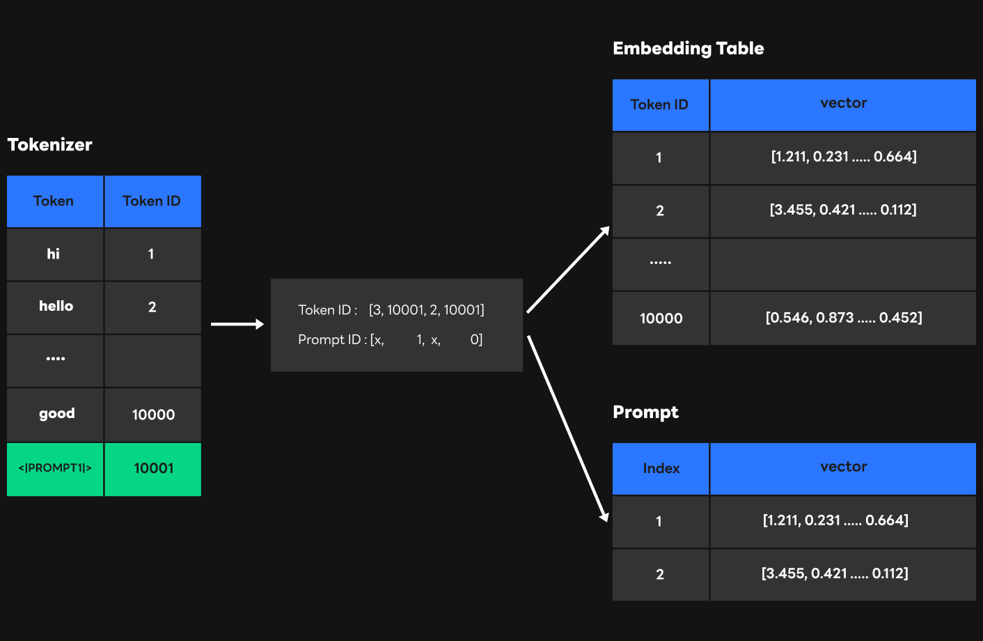
The figure above shows how to deliver prompt information directly at inference time. Unlike the first approach, we allowed the tokenizer to recognize all prompts with one token ID. This certainly helped us prevent performance drop in the tokenizer, but we needed to find a way to distinguish prompts. So we chose to send prompt ID along with the existing token ID to FasterTransformer, and delivered the weight of the prompt that can be indexed with the prompt ID to FasterTransformer together. In this way, FasterTransformer can perform indexing in the embedding table if an ID (1 - 10000) is within the token range trained from the token ID information, and in prompt weight using the prompt ID (10001) when the token ID is out of range (10001).

As a result, using the second approach, we were able to service P-tuning requests within a response time similar to that of normal requests.